

Root Construction
Repeating Proportions from √2 to √8
A painting can contain large and small areas that feel related even when they do not repeat the same subjects. One way to study such relationships is to divide a rectangle into smaller rectangles without changing the underlying proportion. Root constructions provide an exact geometric method for doing this.
The method begins with a rectangle whose longer side is √n times its shorter side. Divide the longer dimension into n equal parts, and every resulting part has the same proportion as the original, rotated by 90°. Repeat the operation on those smaller parts and the proportion returns again and again. The construction can continue to a very fine grid, but its artistic value lies primarily in the relationships between large and small areas.
This article brings together the √2 to √8 constructions in a single sequence. It explains their shared mathematics, the different subdivision depths used in REGIS ARS, and ways to use the resulting grids without mistaking mathematical regularity for artistic quality.
From a square to the family of root rectangles
Begin with a square whose side measures one unit. According to the Pythagorean theorem, its diagonal is √2. Using that diagonal as the longer side and retaining the unit short side constructs a √2 rectangle.
The sequence can continue: a right triangle with legs 1 and √2 has hypotenuse √3. A triangle with legs 1 and √3 produces √4 = 2. Continuing the same process produces √5, √6, √7, and √8. Each new length is geometrically constructible; a decimal approximation is useful for measurements but not the definition of the proportion.
A horizontal root-n rectangle has width W, height H, and:
W/H = √n.
The name describes a side ratio-not a count of lines, cells, or objects. In particular, √4 is exactly 2, so its rectangle is the familiar double square. √8 = 2√2, revealing a useful relationship with the root-two format. Neither √5 nor its subdivisions should be confused with the golden ratio, even though φ = (1 + √5)/2.
Why the subdivision works
Suppose the width of a horizontal root-n rectangle is W = H√n. Divide its longer side into n equal widths. Each new strip is W/n wide and H high. Its longer-to-shorter ratio is:
H/(W/n) = nH/W = √n.
Thus, each strip is a rotated, similar rectangle. Now divide the longer dimension of every strip into n equal parts. This produces n² smaller rectangles oriented like the original. After a third level, there are n³ regions, again rotated. Each level preserves the ratio and divides the area of each parent region equally.
This property is special to the matching root and divisor: a √5 rectangle divided into five strips retains its proportion; divided into six equal strips, it does not. The construction is therefore more than an arbitrary decorative grid.
The procedure has no fixed mathematical stopping point. The subdivision levels shown in REGIS ARS are selected implementation depths, not mandatory limits or historical prescriptions.
Root construction and dynamic symmetry are different guides
Both guides begin with the same family of root rectangles, but they ask different questions:
| Dynamic Symmetry | Root Construction |
|---|---|
| Uses two main diagonals and four perpendicular auxiliary lines, within the outer rectangle | Uses repeated equal divisions of the longer side |
| Reveals diagonal directions, intersections, and reciprocal side areas | Reveals nested proportional regions, repetition, and scale |
| Has a ten-segment framework in REGIS ARS | Has a grid whose density depends on the root and subdivision level |
| Helps compare visual movements and counter-movements | Helps compare large masses, smaller groups, and intervals |
A reciprocal strip one-nth of the parent rectangle’s area appears in both explanations. In Dynamic Symmetry it is revealed through diagonals and perpendiculars; in Root Construction it becomes the *first subdivision step. The geometrical relationship is shared, but the finished guides look different.
Fitting the construction to the canvas in REGIS ARS
REGIS ARS first draws the largest centered root rectangle of the chosen proportion that fits inside the canvas. It then subdivides that fitted rectangle. The program does not stretch a √n construction into an arbitrary canvas aspect ratio.
A 60 × 40 cm canvas, for instance, is a 3:2 rectangle. It is not itself a √2, √3, or √4 rectangle. In this format the √2 guide uses the full 40 cm height, leaving about 1.72 cm on either side. The √3 through √8 guides use the full 60 cm width, leaving equal bands above and below. These uncovered areas remain available for the composition: they are not cropping instructions or errors.
| Root | Ratio (approx.) | Fitted rectangle on 60 × 40 cm canvas | Outer margins |
|---|---|---|---|
| √2 | 1.4142 | 56.57 × 40.00 cm | 1.72 cm left and right |
| √3 | 1.7321 | 60.00 × 34.64 cm | 2.68 cm top and bottom |
| √4 | 2.0 | 60.00 × 30.00 cm | 5.00 cm top and bottom |
| √5 | 2.2361 | 60.00 × 26.83 cm | 6.58 cm top and bottom |
| √6 | 2.4495 | 60.00 × 24.49 cm | 7.75 cm top and bottom |
| √7 | 2.6458 | 60.00 × 22.68 cm | 8.66 cm top and bottom |
| √8 | 2.8284 | 60.00 × 21.21 cm | 9.39 cm top and bottom |
For a portrait canvas, the construction is rotated accordingly. The grid should be interpreted relative to its own fitted boundaries, not automatically as a full-canvas division.
The seven constructions in REGIS ARS
Every level divides the longer dimension of each current region into the number of parts specified by its root. For a horizontal starting rectangle, the directions alternate: vertical divisions first, then horizontal, then vertical again.
| Construction | Subdivision levels | Final regions | Final arrangement (columns × rows) |
|---|---|---|---|
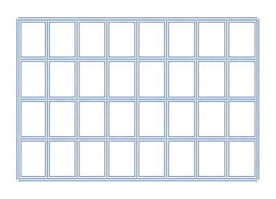
| √2 | 5 | 2⁵ = 32 | 8 × 4 |
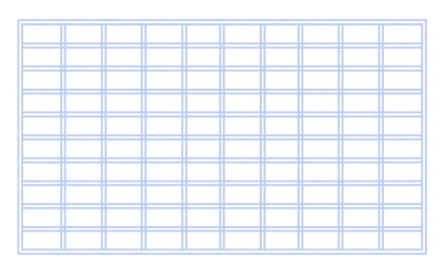
| √3 | 4 | 3⁴ = 81 | 9 × 9 |
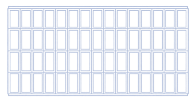
| √4 | 3 | 4³ = 64 | 16 × 4 |
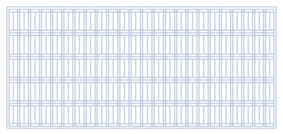
| √5 | 3 | 5³ = 125 | 25 × 5 |
| √6 | 2 | 6² = 36 | 6 × 6 |
| √7 | 2 | 7² = 49 | 7 × 7 |
| √8 | 2 | 8² = 64 | 8 × 8 |
These are numbers of areas, not numbers of drawn lines. The program constructs subdivision segments within parent regions; neighboring segments meet and appear as longer continuous grid lines. The selected subdivision counts control how detailed the visual grid becomes.
√2 – five levels, thirty-two areas
A √2 rectangle is cut into two similar halves. Split both again and there are four areas; three more levels produce 8, 16, and finally 32. The divisions alternate vertical-horizontal-vertical-horizontal-vertical. The finished horizontal construction appears as eight columns and four rows, and its cells are upright root-two rectangles.
On a 60 × 40 cm canvas the fitted region measures approximately 56.57 × 40 cm. Each final cell is about 7.07 × 10 cm. In an illustration, the first central split and the subsequent four-part division are often more useful for explaining the principle than all thirty-two cells at once.
The same proportional behavior is familiar from ideal ISO A-series paper formats, where dividing a sheet in half preserves its approximate aspect ratio. It is a geometric example, not a rule about composition.
√3 – four levels, eighty-one areas
Divide the width into three parts: 3 upright rectangles. Divide those along their longer sides: 9 horizontal rectangles. Repeating the alternating operation gives 27, then 81 similar areas. The final construction appears as a 9 × 9 grid.
Because the grid has equal numbers of rows and columns, it might look superficially like a square-cell grid. It is not: the fitted outer rectangle has √3 proportions, and so does every final cell. Use it to explore changes in grouping and scale, not to impose a conventional Rule of Thirds layout.
√4 – three levels, sixty-four areas
Since √4 = 2, the starting shape is a double square. Dividing it into four equal-width strips produces four upright 2:1 rectangles. The next level creates 16 horizontal rectangles, and the third produces 64 upright rectangles, visible as a 16 × 4 grid.
The first subdivision into four reciprocal strips is different from simply splitting the double square into its two square halves. Both can be useful analytical divisions, but only the four-strip operation gives rotated 2:1 rectangles at the first level.
√5 – three levels, one hundred twenty-five areas
The √5 construction uses five equal divisions at each stage: 5 → 25 → 125 regions. Its final horizontal arrangement is 25 columns by 5 rows. This is the densest of the seven REGIS ARS root-construction guides described here.
The connection to the golden ratio is algebraic- φ = (1 + √5)/2 -not an identity of grids. A √5 subdivision should not be labeled a golden-ratio grid or a Fibonacci construction. In painting, the fine divisions are best used sparingly for checking intervals and repeated accents after larger masses have already been established.
√6 – two levels, thirty-six areas
The first level divides the fitted width into six upright root-six strips. The second divides each strip into six smaller horizontal rectangles, giving 36 areas in a 6 × 6 arrangement. Each small cell has √6 proportions despite the regular row-and-column pattern.
Because the original shape is fairly elongated, examine the outer bands and the ratio between the active group and quieter areas before relying on the complete grid.
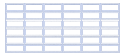
√7 – two levels, forty-nine areas
Seven vertical strips are subdivided into seven horizontal parts each: 7 → 49 regions. The final grid appears as 7 × 7, with each cell preserving the original √7 aspect ratio.
This format makes relatively narrow reciprocal parts visible. It can be useful when comparing a compact group of accents with a broad field, but the number seven does not confer a special universal meaning on their positions.
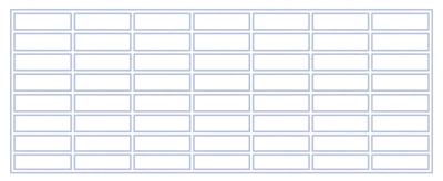
√8 – two levels, sixty-four areas
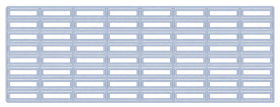
Eight equal vertical divisions followed by eight horizontal divisions produce 64 regions in an 8 × 8 arrangement. Each retains a √8 proportion. Since √8 = 2√2, the undivided root-eight rectangle can also be split into two equal halves, each a horizontal √2 rectangle. This is an additional relationship of the format, not a substitute for the eight-part recursive construction used by the guide.
The √8 format is the most elongated in this sequence. Its internal grid can help compare repeated intervals across a long composition, while the uncovered canvas margins must still be considered.
How to use the grid in painting
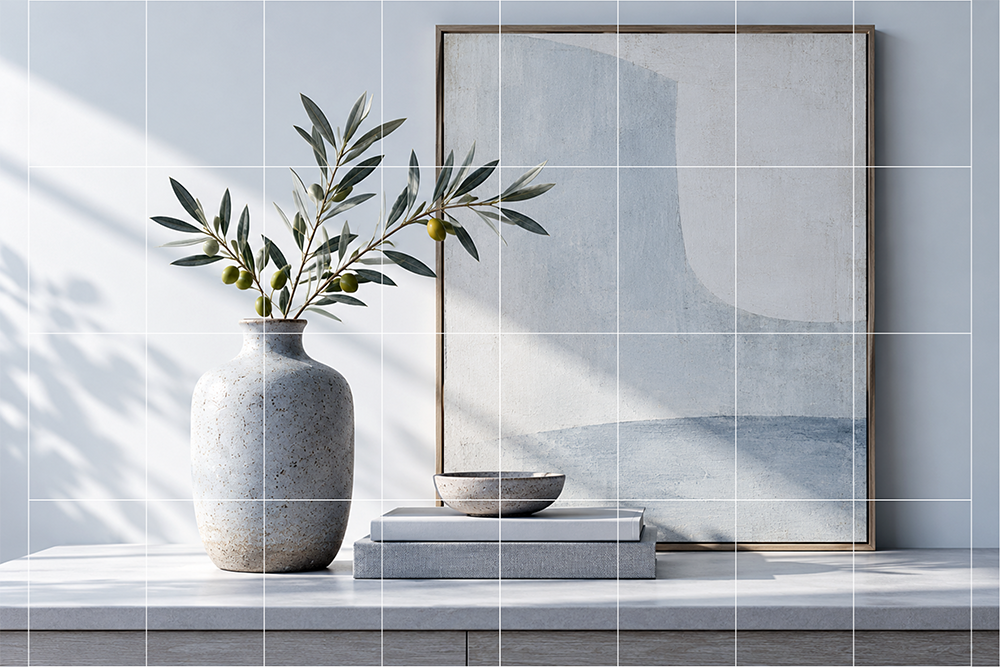
A subdivision grid is most helpful when read from large to small. First examine the outer rectangle and the first split. Decide whether the dominant value mass should occupy one area, cross a boundary, or deliberately counteract the division. Only then turn to finer regions for spacing, scale, and rhythm.
Three distinctions prevent common errors:
- Equal geometric area is not equal visual weight. Contrast, value, saturation, edges, detail, and subject recognition can make one area far more active than another.
- Grid boundaries are not compulsory object boundaries. A figure, tree, shadow, or architectural form may cross several regions. Often that is precisely what makes the composition feel coherent.
- A root grid is not a perspective or anatomical grid. Its divisions do not establish vanishing points, correct head proportions, or a mandatory horizon height.
A useful strategy is to combine several adjacent cells into one major dark or light mass, leaving another group quieter. What matters is the relationship of shapes, not how many individual cells are visibly occupied.
Practical exercise: from a simple split to the complete grid
Choose a subject with two or three clear masses and work at the same canvas dimensions throughout. Compare four small studies:
- Without a grid. Establish the major value masses and negative space by eye.
- With the first subdivision. Use two, three, four, or more large regions depending on the chosen root. Decide where the dominant group belongs.
- With the complete grid. Use finer divisions to assess intervals and repeated shapes, but avoid placing an object in every cell.
- With the grid hidden. Revise the study for clarity and expressive intent. Remove any alignment that weakens the image.
Try the same subject first with √2 and then with √5. The grids differ greatly in density, even though both use the same self-similarity principle. Compare the outcome at thumbnail size before deciding whether the additional divisions were helpful.
Historical context and limitations
Root rectangles arise from elementary geometry and can be constructed independently of any historical theory of art. Jay Hambidge developed influential arguments about root proportions and dynamic symmetry in the early twentieth century. Later geometric studies, including those of Rachel Fletcher, examined these rectangles as design constructions. However, a mathematically correct overlay is not evidence that a particular historic painter used it.
The subdivision depths listed above describe the REGIS ARS implementation, not a fixed rule passed down from ancient Greece. A painter can examine fewer levels, ignore individual divisions, or abandon the overlay entirely when observation leads to a stronger result.
Conclusion
Root Construction √2–√8 is a family of self-similar proportional grids. Each root determines how many strips preserve the parent ratio; successive levels build a hierarchy from large areas to smaller ones. The seven versions differ in aspect ratio and grid density, but they teach one common lesson: precise subdivision can clarify relationships, while visual balance remains the artist’s responsibility.
For diagonal and reciprocal frameworks using these same proportions, see Dynamic Symmetry: √2–√8.
Sources and further reading
1. Hambidge, Jay. The Elements of Dynamic Symmetry. Brentano’s, 1926.
2. Fletcher, Rachel. Dynamic Root Rectangles. Part One: The Fundamentals. Nexus Network Journal 9(2), 2007, pp. 327–361.
3. Fletcher, Rachel. Dynamic Root Rectangles Part Two: The Root-Two Rectangle and Design Applications. Nexus Network Journal 10(1), 2008, pp. 149–178.
4. Blake, Edwin M. Dynamic Symmetry-A Criticism. The Art Bulletin 3(3), 1921, pp. 107–127.
5. ISO. ISO 216:2007: Writing Paper and Certain Classes of Printed Matter-Trimmed Sizes.